Review of Digital Image Orthorectification Techniques

Dr. F. I. Okeke
Department of Geoinformatics and Surveying,
University of Nigeria, Enugu Campus, Nigeria

Introduction
Aerial photos and satellite images do not show features in their correct locations due to displacements caused by the tilt of the sensor and terrain relief. Orthorectification transforms the central projection of the photograph into an orthogonal view of the ground, thereby removing the distorting effects of tilt and terrain relief. Orthorectification is the process of transforming raw imagery to an accurate orthogonal projection, as against the perspective projection of the raw image (Fig 1). The product of orthorectification process is orthoimage or orthophotos. Without orthorectification, scale is not constant in the image and accurate measurements of distance and direction cannot be made.

Fig.1: Orthogonal vs. perspective projections

In order to orthorectify imagery, a transformation model is required which takes into account the various sources of image distortion generated at the time of image acquisition. These include:

• Sensor orientation
• Topographic relief
• Earth shape and rotation
• Sensor orbit and attitude variations
• Systematic error associated with the sensor

The required geometric parameters regarding sensor orientation at the time of image acquisition are determined through information on the sensor model, Ground Control Points (GCPs), and platform orbital or flight data (position, velocity, orientation).

Because orthoimages are planimetrically correct, it can be an effective tool for use in resource management, municipal planning, cadastral mapping, and geographic information systems (GIS). It is not only true in scale and area, but like a conventional aerial photograph it is easily interpreted. A forester in the field of resource management can designate and outline forest-type boundaries on an orthophoto directly.

However, the conventional orthorectification processes do not take into account objects that mathematically can be described like buildings, bridges, trees etc. Such objects remain in perspective views in the resulting orthophotos and are distorted from their true positions. Distortions show as, for instance, leaning buildings and bent bridges. Some interesting information from ground features like streets and other objects are hidden from the user of the orthoimage. Furthermore the superimposition of vector data is nearly impossible. If Digital Surface Models (DSMs) describing the mentioned objects that caused the displacement are used for the orthorectification processes, the displacements can be corrected and the results are called “True Orthoimages”.

This article however reviews only some of the conventional digital orthorectification techniques.

Orthorectification algorithms
Generally there are two classes of rectification approaches. The parametric and the non-parametric approaches (Hemmleb and Wiedemann, 1997). Whereas for the parametric approach the knowledge of the interior and exterior orientation parameters is required, non-parametric approaches require just control-points. Non-parametric approaches include polynomial transformation, and projective transformation. A comprehensive comparative study of orthorectification approaches can be found in Novak (1992).
Polynomial rectification
The simplest way available in most standard image processing systems is to apply a polynomial function to the surface and adapt the polynomials to a number of checkpoints (GCPs). The procedure can only remove the effect of tilt, and can be applied on both satellite images and aerial photographs. One of several polynomial orders may be chosen, based on the desired accuracy and the available number of GCPs. Rosenholm and Akerman (1998) stated that for satellite images with simple geometric conditions, such as, near vertical and/or relatively flat areas, a low degree polynomial can give a sub-pixel result, and that higher degree polynomials are unreliable. Also Novak (1992) concluded that although polynomial rectification algorithm is very easy to use, they do not adequately correct relief displacement. Hemmleb and Wiedemann (1997) observed that it seems to be very dangerous to use higher grade polynomial transformations for the rectification of images, and that the required amount of control points and the risk of an oscillation is growing with the grade of the polynomial. Polynomial rectification equations are given by equations 1, and 2, below.

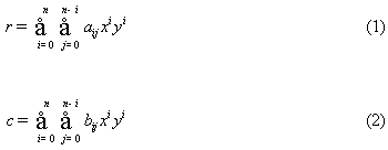
Where r, c are pixel coordinates of input image (row and column); x, y are coordinates of output image; a, b are coefficients of the polynomial, and n is the order of the polynomial.

Projective rectification
To perform a projective rectification, a geometric transformation between the image plane and the projective plane is necessary. For the calculation of the eight unknown coefficients of the projective transformation, at least four control points in the object plane are required. Projective transformation is applicable to rectifying aerial photographs of flat terrain or images of facades of buildings, since it does not correct for relief displacement (Novak, 1992). The equations for projective rectification are given as follows (Hemmleb and Wiedemann, 1997):

Where r, c are pixel coordinates of input image (row and column); x, y are coordinates of output image; b11 L b23 are coefficients.

Differential rectification
The objective of differential rectification is the assignment of grey values from the image (usually aerial image) to each cell within the orthophoto. Differential rectification is a phased procedure that uses several XYZ control points to georeference an image to the ground. Novak (1992) pointed out that the differential rectification corrects for both relief displacement and camera distortions, yields the best results, and can be applied for both aerial and satellite imagery.

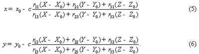
The procedure of differential rectification is applied in combination with the back projection (indirect) method of orthoimage reprojection (see section 3 below). This is based on the well-known collinearity principle, which states that the projection center of a central perspective image, an object point, and its photographic image lie upon a straight line. The collinearity principle is described by means of equations (5) and (6) (Kraus, 1992):

Where:

• (x,y) are the coordinates of the point object in the image space
• (x0,y0) are the image coordinates of the calibrated principal point (point of symmetry) of the camera;
• c is the calibrated camera focal length;
• (X0,Y0,Z0) are the coordinates of the camera station, and
• w,j,k are the rotation angles between the image coordinate system and the ground coordinate system
• rij are the elements of the rotation matrix between the image and ground systems.

The procedure of differential orthorectification is as follows (Mayr and Heipke, 1988):

• Define a uniform grid over the orthophoto plane (datum).
• For each grid element (X, Y) in the orthophoto plane interpolate for the corresponding elevation Z(X, Y).
• Using the external orientation parameters (EOP) and internal orientation parameters (IOP) together with the collinearity equations find the corresponding image point (x, y).
• Find the gray value g(x, y) using one of the resampling techniques.
• Repeat the above procedure for all the pixels in the orthophoto plane.

Sensor model rectification
Sensor models are required to establish the functional relationship between the image space and the object space. Sensor models are typically classified into two categories: physical and generalized models. The choice of a sensor model depends primarily on the performance and accuracy required and the camera and control information available (Tao and Hu, 2001). A physical sensor model represents the physical imaging process. The parameters involved describe the position and orientation of a sensor with respect to an object-space coordinate system. Physical models, such as the collinearity equations, are rigorous, very suitable for adjustment by analytical triangulation and normally yield high modeling accuracy (a fraction of one pixel).

There are many types of sensors such as Frame, Pushbroom, Whiskbroom, Panoramic, and SAR, etc. Physical models are sensor dependent where each requires a unique sensor model. With the increasing availability of imaging sensors, from an application point of view, it is not convenient for users to change the software or add new sensor models into their existing system in order to process new sensor data. Moreover, for dynamic sensors, the physical parameterization may become much more complicated since the orientation parameters vary with time and must be expressed as a function of time over the imaging period. It is also realized that rigorous physical sensor models are not always available, especially for images from commercial satellites (e.g., IKONOS), where the rigorous sensor models are hidden to the end users. This causes difficulties in developing a rigorous sensor model without knowing its imaging parameters (e.g., imaging geometry, relief displacement, Earth curvature, atmospheric refraction, lens distortion, etc.). The physical sensor models are mathematically complex and usually require relatively long computation time.

Rigorous physical sensor models are more accurate (Rosenholm and Akerman, 1998; Tao and Hu, 2001). An example is the orbital model of the satellite track and the rotation angles of the instrument for orthorectification of IRS images (Rosenholm and Akerman, 1998). However the development of generalized sensor models independent of sensor platforms and sensor types is very attractive. In a generalized sensor model, the transformation between the image and the object space is represented as some general function without modeling the physical imaging process.

Rational function model rectification
Generalized sensor models, such as the usage of the Rational Function sensor Model (RFM) (Tao and Hu, 2001), have alleviated the requirement to obtain a physical sensor model, and with it, the requirement for a comprehensive understanding of the physical model parameters. Furthermore, as the RFM sensor model implicitly provides the interior and exterior sensor orientation, the availability of GCPs is no longer a mandatory requirement. Consequently, the use of the RFM for photogrammetric mapping is becoming a new standard in high-resolution satellite imagery. This has already been implemented in various high-resolution sensors, such as IKONOS and QuickBird (Croitoru et al., 2004).

The RFM sensor model describes the geometric relationship between the object space and image space. It relates object point coordinates (X,Y,Z) to image pixel coordinates (r,c) or vice versa using 78 rational polynomial coefficients (RPCs). For the ground-to-image transformation, the defined ratios of polynomials have the following form (Croitoru et al., 2004):

Where (rn,cn) are the normalized row (line) and column (sample) index of pixels in image space; Xn) ,Yn) and Zn) are normalized coordinate values of object points in ground space; and the polynomial coefficients aijk, bijk, cijk, are called Rational Function Coefficients (RFCs).

Orthorectification reprojection
Orthorectification algorithms are often performed in conjunction with reprojection procedure, where rays from the image are reprojected onto a model of the terrain. Fundamentally reprojection can be done in two ways:

• Forward projection or direct projection
• Backward projection or indirect method

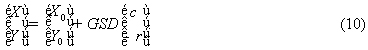
In the first case of forward projection, the pixels from the original image are projected on top of the DEM of the 3D model and the pixels’ object space coordinates are calculated. Then, the object space points are projected into the orthoimage. Because of the gap between the points projected into the orthoimage, due to the terrain deviation and perspective effects, the forward projection projects regularly spaced points in the source image to a set of irregular spaced points. Therefore they have to be interpolated into a regular array of pixel that can be stored in a digital image. This is why the backward projection is often preferred (Mikhail et al., 2001). If the corner of the orthoimage is placed at X0) ,Y0) , the pixel coordinate column and row,(c,r) in the orthoimage is found by (Mikhail et al., 2001):

Where GSD is the Ground Sample Distance, which is the distance between each pixel, also referred to as the pixel size. Notice that the equation takes into account that pixel coordinate system has the Y-axis downwards and the world coordinate system has the Y-axis pointing upwards/north.

In the case of backward projection, the object space X, Y coordinates related to every pixel of the final orthoimage are determined. The height Z at a specific X, Y point is calculated from the DEM or the 3D model and then the X, Y, Z object space coordinates are projected in the original image in order to acquire the gray level value for the orthoimage pixel. Interpolation or resampling process in the original image is also essential because of the fact that the projected coordinates will not fit accurately at the original image pixel centers. In the backward projection instead of interpolating in the orthoimage, the interpolation is done in the source image. This is easier to implement, and the interpolation can be done right away for each output pixel. Further more only pixels that are needed in the orthoimage are reprojected. In the backward projection method, the pixel-to-world transformation is again given by (Mikhail et al., 2001) as

The position in the same image that corresponds to the found XYZ can be obtained by a sensor model (i.e collinearity equations as applied in the differential orthorectification method).

General orthorectification workflow
Most commercial off-the-shelf software (COTS) for software (i.e Erdas Imagine, PCI Geomatics, ENVI, ZI Imagine, LH System, TNT products, etc) contain comprehensive suite of products designed for performing tasks required in producing high quality, seamless digital orthophoto imagery products from aerial (standard and digital) and commercial satellite imagery. These software products include programs required to produce the input components for orthorectification including project setup, DEM interpolation/formatting, and GCP and tie point collection. These products can also be used to create imagery mosaics, and they have the ability for orthorectification using RPFs

Most of these software products currently support processing of ephemeris data and orthorectification for the following commercial imaging satellites:

• Landsat 4, 5 and 7
• SPOT 1,2,3, and 4
• IRS 1-A, 1-B, 1-C, and1-D
• AVHRR
• ASTER
• Ikonos
• Quickbird

In these software, project setup requires the user to specify project, name, input and output projections, formats (i.e. what projection the GCPs are being collected in), whether aerial or satellite modeling, type of sensor, etc.) Depending on the availability and format of the control points and the method used, GCPs can be input using a variety of methods including extraction from geocoded images and vector files, importing from text files and captured from hardcopy sources using a digitizing tablet. A minimum of four GCPs is required for each satellite image, although six to eight are recommended.

Tie points are produced by identifying the same pixel location in two or more images within their overlap areas. These software products can process tie points for an unlimited number of input images.

To get an overview of the control point residuals and identify possible outliers, these software provide the ability to generate residual reports for all scenes within a project or for individual scenes.

Mosaicking requires delineation of cutlines and, in many cases, radiometric adjustment of adjacent images to hide the seamlines and produce a more visually pleasing product. These software have both manual and automatic mosaicking options.

General orthorectification workflow includes the following tasks:

1. Importing raw satellite imagery, including orbital metadata for a variety of airborne cameras and sensors
2. Collecting ground control points from an existing geocoded images
3. Refining the collected ground control points based on criteria such as high residual error
4. Calculating the updated model for the images with the refined GCPs
5. Given the model and a DEM (or an approximate elevation), generate the orthorectified images

Conclusion
This article has described, in a succinct form, some of the popular conventional techniques of orthorectification. These methods range from those with simple algorithm to those with sophisticated routines, such as the physical and the generalized models. Modern trend has shown more inclination to the use of generalized models. One of such state-of-the-art method is the application of RFM. In future RFM will have the advantage that the photogrammetric processing software can be kept unchanged when dealing with different sensor data since the generalized sensor model is sensor independent. For new sensors, only the values of coefficients in the generalized sensor model need to be updated.

Again since there are no functional relations between the parameters of the rigorous model and those of the RPF, the physical parameters cannot be recovered from the RPF and the sensor information can be kept confidential. Currently, in order to protect the undisclosed sensor information, some commercial satellite data vendors, such as Space Imaging Inc., only provide users with the RFM parameters but do not provide any information regarding the physical sensor model. Even under this condition, users are still able to achieve a reasonable accuracy without knowing the rigorous sensor models for photogrammetric processing.

References

• Croitoru, A. et al., (2004). “The Rational Function Model: A Unified 2d And 3d Spatial Data Generation Scheme”. Proceedings of ASPRS Annual Conference, Denver, Colorado, USA
• Hemmleb, M. and Wiedemann, A., (1997). “Digital Rectification and Generation of Orthoimages in Architectural Photogrammetry”. CIPA International Symposium, IAPRS, XXXII, Part 5C1B: 261-267, Göteborg, Sweden,
• Kraus, K., (1992). “Photogrammetry Fundamentals and Processes”. Dummler Verlag, Bonn.
• Mayr, W. and Heipke, C., (1988). “A Contribution to Digital Orthophoto Generation.” International Archives of Photogrammetry and Remote Sensing, 27, Part B11-IV: 430 – 439.
• Mikhail, E.M., Bethel, J.S. and McGlone, J.C., (2001). “Introduction to Modern Photogrammetry.” Wiley, New York.
• Novak, K., (1992). “Rectification of digital imagery”. Photogrammetric Engineering and Remote Sensing, 58(3): 339-344.
• Rosenholm, D. and Akerman, D., (1998). “Digital Orthophotos from IRS – Production and Utilization”. GIS – Between Visions and Applications, ISPRS, 32, Stuttgart, Germany
• Tao, C.V. and Hu, Y., (2001). “The Rational Function Model: a tool for processing high resolution imagery”. Earth Observation Magazine (EOM), 10(1).