
Introduction
The paper focuses on use of remote sensing and Light Detection and Ranging (LiDAR) technology in understanding the archaeology in Brazil, primarily in City of Rio de Janeiro. Archaeologists who have not studied the physical principles of remote sensing do not use the full capacity of this technology and thus generate wrong data.
Experiences and perceptions in Rio de Janeiro
Archaeologists who have not studied the physical principles of remote sensing do not use the full capacity of this technology vis a vis archeology and thus generate wrong data. For many archaeologists remote sensing is too technical. Archaeologists must delve into reflectance studies, radiation issues / received and absorption. Thus, under the Brazilian framework July 2012 there are three categories of research and management: government, university and private area. The difference in applicability in management or research is significant. Spectral Range (μm) has a utility to decisions: A.Archaeological Research 0.45 to 0.52 (Blue): Map Coastal Waters, Differentiated: Soil and Vegetation and Differentiate: Coniferous and deciduous. B. Archaeological Management: 0.76 to 0.90 (Near Infrared): Outline Water Bodies, Geomorphological mapping, Geological Mapping, Burned Areas, Wetlands, Agriculture and Vegetation in Electromagnetic Spectrum.
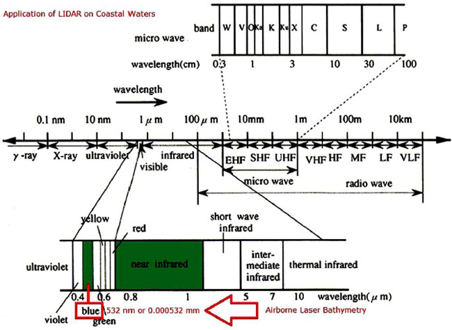
Electromagnetic Spectrum © Carlos Eduardo Thompson Alves de Souza
Airborne Laser Scanning (ALS) of urban regions is nowadays commonly used as a basis for 3D modeling of the urban archaeology. Laser scanning has several advantages as compared to classical aerial photography. It delivers direct 3D measurements independently from natural lighting conditions, and it offers high accuracy and point density. Despite increasing performance of LiDAR systems, most remote sensing tasks that require on-line data processing are still accomplished by the use of conventional CCD or infrared cameras.
Methodology
In this study the area was analysed by airborne laser scanning of the archaeological site of the low visibility within the Catacumba Municipal Park, an Urban Site of the South Zone of Rio de Janeiro.
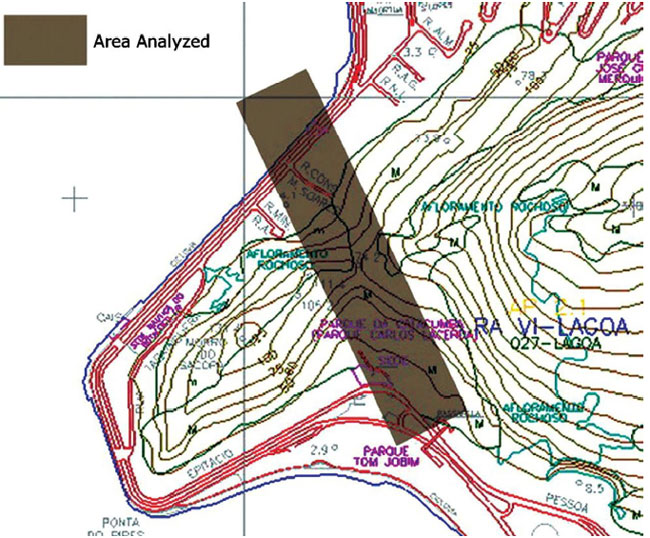
Map of the Catacumba Municipal Park © Carlos Eduardo Thompson Alves de Souza

Catacumba Municipal Park © Carlos Eduardo Thompson Alves de Souza
Under the archaeological workflow of ALS data processing, the first step is to register all the collected data by using navigational sensors, resulting in an irregularly distributed 3D point cloud. Automatic processing of these data is quite complex since it is necessary to determine a set of nearest neighbors for each data point to handle search operations within the data set. In Brazilian archaeology we call these data with “Plan of Work”. The common technique for that is the generation of a Triangulated Irregular Network or TIN. This approach leads to most accurate results, but it is not applicable for real-time applications. Most of currently used airborne laser scanners like the RIEGL LMS-Q560 utilise opto-mechanical beam scanning to measure range values in single scan lines. The third dimension is provided by the moving airborne platform. To fast pre-classification of LiDAR points and segmentation of archaeological sites in urban environments based on the analysis of these scan lines. Instead of initial georeferencing of all range measurements, the analysis of geometric features in the respective local neighborhood of each data point is performed directly on the 2D regularly distributed scan line data. These operations can be executed comparatively fast and are applicable for online data processing. If an accurate city model is already available, the proposed methods could be used for a structural comparison, e.g. for archaeological sites detection. Two major classes of segmentation algorithms can be pointed out: surface growing and scan line segmentation.
The RIEGL LMS-Q560 is a laser scanner that gives access to the full waveform by digitising the echo signal. The sensor makes use of the time-of-flight distance measurement principle with nanosecond infrared pulses. Opto-mechanical beam scanning provides single scan lines, where each measured distance can be geo-referenced according to the position and orientation of the sensor. Waveform analysis can contribute intensity and pulse-width as additional features, which is typically done by fitting Gaussian functions to the waveforms. Since we are mainly interested in fast processing of the range measurements, we neglect full waveform analysis throughout this paper. Range d (expressed in meter) under scan angle α (-30 degree to 30 degree) is estimated corresponding to the first returning echo pulse as it can be found by a constant fraction discriminator (CFD). Positions with none or multiple returns are discarded, and with x=d•sin (α), y=d•cos (α) the scan line data is given in 2D Cartesian coordinates. Since the rotating polygon mirror operates with 1000 scan positions, one scan line can successively be stored in an array A. The navigational data assigned to each range measurement need also to be stored in that array for later georeferencing. If we have a set of n points {p1, …, pn} and we assume that this set mostly contains points that approximately lie on straight line (inliers) and some others that do not (outliers), simple least squares model fitting would lead to poor results because the outliers would affect the estimated parameters. To compute a straight line, a random sample of two points (the minimal subset) pi and pj is selected. The resultant line’s normal vector n0 can easily be computed by interchanging the two coordinates of (pi – pj), altering the sign of one component and normalising the vector to unit length. This yields the normal vector n0 and with (x–pi) •n0 = 0 the line. If the distance d is below a pre-defined threshold, we assess that point as inlier. The number of inliers and the average distance of all inliers to the line are used to evaluate the quality of the fitted straight line. This procedure is repeated several times in order to converge to the best possible straight line.

Airborne Platform © Carlos Eduardo Thompson Alves de Souza
The following steps are executed to fit straight line segments to the scan line data and to remove irregularly shaped objects: (1) Choose an unmarked position i at random among the available data in the array a holding the scan line data. (2)Check a sufficiently large interval around this position i for available data, resulting in a set S of 2D points. (3) Set the counter k to zero. (4) If S contains more than a specific number of points (e.g. at least six), continue. Otherwise marks the current position i as discarded and go to step 14. (5)Increase the counter k by one.(6) Perform a RANSAC-based straight line fitting with the 2D points in the specified set S. (7) If RANSAC is not able to find an appropriate straight line or the number of inliers is low, mark the current position as discarded and go to step 14. (8) Obtain the line’s Hessian normal form (x–pi) •n0 = 0 and push the current position i on an empty stack. (9) Pop the first element j off the stack. (10) If the counter k has reached a predefined maximum and the number of points in S is high enough, store the 2D normal vector information n0 at position j and mark that position as processed. (11) Check each position in an interval around j that has not already been looked at whether the respective point lies sufficiently near to the straight line. If so, push its position on the stack. Additionally, include the 2D point in a new set S’. (12) While the stack is not empty, go to step 9. Otherwise continue with step 13. (13) If the counter k has reached its maximum (e.g. two cycles), set it to zero and continue with step 14. Otherwise go to step 4 with the new set of points S: =S’. (14) Go to step 1 until a certain number of iterations has been performed or no unmarked data is available in the scan line. In each iteration step we randomly select a position in the array A of scan line data points and try to fit a straight line segment to the neighboring data at that position. If the fitted straight line is of poor quality, the data associated with the current position is assessed as clutter. Otherwise, we try to optimize the line fitting by looking for all data points that support the previously obtained line, which is done in steps (9), (10), (11) and (12). These steps actually represent a line growing algorithm. The local fitting of a straight line segment is repeated once with the supporting points to get a more accurate result. The end points of the resulting line segment can be found as the perpendicular feet of the two outermost inliers. These and the 2D normal direction are stored before the method is repeated until all points in the scan line are either assessed as clutter or part of a line segment.
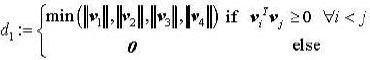
The next step is to identify all points in the scan line that form the ground level. A line segment at ground level can be characterized by the number of points lying beneath it in an appropriate neighborhood with respect to its 2D normal direction (that number should be near zero). In general, this is not a sufficient condition, but it yields enough candidates for an estimation of the dividing line between objects of interest and ground level. The dividing line is formed by estimates of the sensor-to-ground distance in y-direction at each position in the scan line. Each newly found line segment, potentially lying at ground level, contributes to that estimate in a neighborhood of its position with respect to its normal direction. Thus, this approach is permissive to unevenness of the terrain. Finally, all line segments lying completely below the dividing line are assessed as ground level, whereas line segments crossing or lying above are classified as part of a building. For increased robustness, the exponentially smoothed moving averages of the dividing line’s parameters are perpetually transferred from the previously processed scan lines. Detected straight line segments within a single scan line are often ambiguous and affected by gaps. To merge overlapping or adjacent pieces that are collinear, line-to-line distances have to be evaluated. Let (P1, P2) and (Q1, Q2) denote two different line segments detected within the same scan line.P1, P2, Q1, and Q2 are the georeferenced end points in 3D space. Since every range measurement has a time-stamp, P1 and Q1 can be chosen to represent the first recorded end point in the respective line segment, P2 and Q2 are chosen accordingly. Two different distance measures are evaluated to decide whether the two line segments are to be merged or not. The first distance d1 indicates if (P1, P2) and (Q1, Q2) are overlapping. In that case it would be zero; otherwise it is set to the minimum Euclidean distance between end points of the two line segments. With the abbreviations v1 = p1 – q1, v2 = p1 – q2, v3 = p2 – q1, and v4 = p2 – q2, distance d1 is defined as
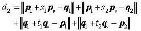
With pv = (p2 – p1)/|| p2 – p1|| and qv = (q2 – q1)/|| q2 – q1||, the parameters of the perpendicular feet of each end point with respect to the other line segment are given as
s1 = (q1 – p1)T pv t1 = (p1 – q1)T qv
s2 = (q2 – p1) T pv t2 = (p2 – q1) T qv
The second distance d2 is a measure of collinearity. It describes the sum of all minimal Euclidean distances of end points to the other line segment. Using the above parameters s1, s2, t1 and t2, distance d2 can be expressed as
Let L denote the list of all detected line segments within the current scan line. The algorithm to find corresponding line segments works as follows: (1) Initialize the current labeling number m with 1. (2) Select the next entry a in L, starting with the first one. (3) If a is unlabeled, set its label to m and increase m by 1. (4) Successively test each line segment b in L following after a if d1 (a, b) and d2 (a, b) are smaller than predefined thresholds. If so, go to step (5), otherwise continue with testing until b reaches the end of the list L. In that case, go to step (6) (5) If b is unlabeled, set its label to the label of a. Otherwise set the label of a and b to the minimum of both labels. Continue testing in (4). (6) Continue with (2) until a reaches the end of the list L. (7) Repeat the procedure until labels do not change anymore. Roughly spoken, the above procedure first initializes each line segment detected in the scan line with a unique label. Those collinear line segments that are found to overlap or lie adjacent are linked together by labeling them with their minimum labeling number. This process is repeated until the labels reach a stable state. The emerging clusters of line segments with same label are then represented by one single line segment, given by the two outermost end points of that cluster. In principle, merging of 3D line segments over multiple scan lines is performed similar to the methods described in the previous section. In contrast to merging of line segments within the same scan line, we are now interested in coplanarity instead of collinearity. Thus other distance measures have to be evaluated. Let Pi, Pj, and Pk be three of the four end points of two line segments. The distance of the fourth end point Pm to the plane defined by the three others is a measure of coplanarity. We define distance d3 as the sum of all four possible combinations:
With the notations, d4 is simply defined as the minimum Euclidean distance between respective first and last end points and the centers of two line segments
Another distance measure can be expressed by the angle between direction vectors pv and qv
Labeling of line segments over multiple scan lines works analogous to the labeling procedure within a single scan line. Nevertheless, there are some differences since scan lines are recorded successively. Moreover, simply testing of two line segments for coplanarity would allow the label to be handed over at edges of buildings. To avoid that, the 3D normal direction at each line segment has to be estimated. Let n be the number of scan lines to be traced back (e.g. five). L0 denotes the list of line segments in the current scan line, L1 is one scan line behind, L2 is two steps behind and so forth. First, test every line segment in L0 if it is near to other line segments in {L1, Ln} in terms of distance measures d3, d4, and d5. If line segments a and b correspond this way, store this link in a database. After that, line segments in Ln will receive no further links. The 3D normal direction at each line segment in Ln is estimated by RANSAC based plane fitting to the set of associated other line segments. If that set contains too few points or the number of outliers is high, the respective line segment is of class 2. Those line segments are typically isolated or near to the edge of a building. All other line segments in Ln belong to class 1 and a 3D normal direction can be assigned to them. Initialize all line segments of Ln with new labeling numbers. Test every line segment in Ln if it is near to other line segments in {Ln+1, …, L2n} in terms of distance measures d3, d4 and d5 (these links are already established). If line segments a and b are linked, the following cases may occur: 1. a and b are of class 2: do nothing only one line segment is of class 1: the class 2 line segment receives the label of the class 1 element; 2.a and b are of class 1: if the angle between the associated normal directions (calculated same as d5) falls below a predefined threshold, set the label of a and b to the minimum of both labels. Continue comparing Ln to {Ln+1, L2n} until labels reach a stable state. Just for clarification: the labels that are assigned to the scan lines in section 3.4 are independent from those introduced here. The first n scan lines are required for initialization before the algorithm starts working. At least 2n scan lines are needed before the merging of line segments begins. Line segments that form a connected (mostly planar) surface will successively be marked with the same label until no more fitting line segments are recorded. For data storage and preparation of subsequent analysis, it is convenient to delineate each completed cluster of connected line segments by a polygon (closed traverse). The 3D normal direction nc of a cluster C can be estimated as the weighted average of normal directions of all line segments (weighted by line length). It is easy to determine an affine transformation E that transforms nc to the z-axis, such that the points of E(C) roughly lie in the x-y plane. The boundary is derived by determination of a 2D alpha shape with an alpha corresponding to scan line distance. The basic idea behind an alpha shape is to start with the convex hull. Then a circle of radius α is rolled around that convex hull. Anywhere the alpha-circle can penetrate far enough to touch an internal point (a line segment) without crossing over a point at the boundary, the hull is refined by including that interior point. Then the alpha shape is transformed back by application of E-1. Finally, we have a set of 3D shapes representing grouped line segments resulting from scan line analysis. Subsequent analysis depends on the problem at hand. For building reconstruction and model generation, the detected planar faces have to be intersected to find edges and corners.
Underwater archaeology & air light detection and ranging
Underwater archeology in the collection of information bathymetry and sound is made by an echo sounder hydrographic resolution 0.01 m and frequency 200 Hz, with door to Side-Scan Sonar (side scan 15 and 20m) and receiver attached to it, carried in a boat fiber (Neves da Fonceca, L.E., 1999).The overall goal is to apply the technology”s potential ALS in the planning and design projects with emphasis on Underwater Archaeology Archaeological Management. The specific objectives are the generation of the Land Surface from data from the ALS technology, evaluate the ALS technology in technical planning and spatial management of a set of sites with the same marker Cultural Creation of a Digital Elevation Model; Valuing Integrated with the Interest of Local Societies and the Natural Resources and contribute to the knowledge and dissemination of technology ALS. Side Scan Sonar (Sounding Navigation and Ranging) systems are active remote sensing, emitting waves and record to produce acoustic images (sonographic records) of the seafloor. These records contain measurements of the acoustic energy that returns to the electroacoustic transducer (Fish, 1990). The geometry of the acquisition sonographic data has many similarities with data from side-looking radar. The LIDAR system is also capable of surveying underwater relief through Bathymetric LIDAR. This system measures the depth of laser beams by shining high-power water. Infrared beams are used, which are reflected by the surface of water, and green beams, which penetrate the liquid layer reflecting in the background. The depth is calculated by the interval of response of the receiver beams. The phenomena of absorption, diffraction and refraction limit the maximum detectable depth, being around 20 to 30 meters with a precision bathymetric approximately 15cm. For a higher density of sampling points, operating at low altitudes and speeds. The turbidity of the water in certain parts of the coast of Rio de Janeiro is a limiting factor in the efficient use of the system. The water/air interface and the seabed generate spikes in the intensities of the returning light from the green laser pulse. The position of the reflecting surface and the intensity can be calculated from these spikes. The position of the water surface is known from the infrared laser measurements and, the depth of the water can be calculated by measuring the time difference between the surface return and the bottom return from the green laser ( Anders Ekelund, Airborne LiDAR Systems for Land and Sea-floor Surveys ).
As the green laser travels through the water and reflects off the seabed, it is subjected to refraction, scattering and absorption. These processes cause attenuation of the laser and limit the depth of water that can be measured. Water that is murky or has high particle content creates the problem of high backscattering from the water column. Backscattering of the laser pulse limits the amount of light which can reach the seabed and at some point makes it impossible to distinguish the backscatter from the bottom return. The identification of the correct position of the top and bottom return is important to accurately determine the water/air interface and the seabed. The maximum depth for ALB is determined by the reflective characteristics of the seabed and water clarity. Under ideal conditions the theoretical maximum depth measurement is 70 m (( Anders Ekelund, Airborne LiDAR Systems for Land and Sea-floor Surveys).
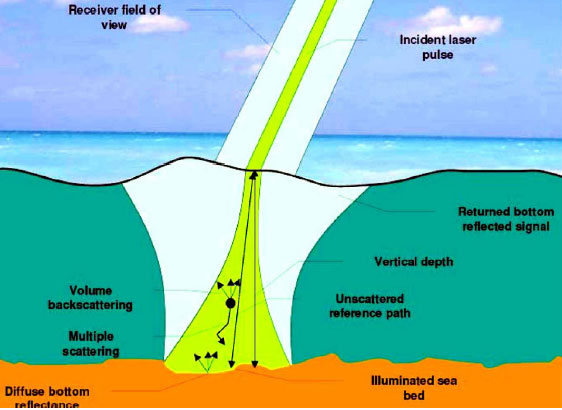
Schematic Diagram of Scattering Effects© Carlos Eduardo Thompson Alves de Souza
Often the specified measurable depth by ALB systems refers to a factor in relation to depth. The method of measuring water clarity. depth in Rio de Janeiro is determined by the use of a circular 20cm diameter plate with alternating black and white quadrants. The disk is attached to a measuring line or pole, which is lowered into the water and the depth at which the disk disappears from view, is noted. The disk is further lowered, and then raised until it comes into view again. The depth is again noted. The depth is the average of these two depths. Acquisition geometry includes the swath width and the footprint size. The swath width is the across track distance covered by each single scan line. The footprint size is the area on the sea bed which is covered by each individual laser pulse. The scan angle is the angle from nadir to maximum scanned angle. In ALB the swath width and the footprint size are dependent on the scan angle. The footprint size of the laser increases with depth due to scattering and refraction in the water column, however this is not nearly to the same degree as in MBES. The small changes in ALB footprint size over varying depths means that the swath width can remain constant without adversely affecting the point density. If the altitude of the aircraft needs to be changed to be able to fly below clouds or turbulent airspace, the scan angle can be widened to maintain the same swath width and footprint size. Advantages& Disadvantages of ALB. A. Advantages: The ability to survey the combined features and constructions, both above and below the waterline in a single scan. In addition, detailed digital images are recorded to allow for visual analysis and use with digital terrain models. The ability to survey closes to shore in areas where it would be dangerous or inaccessible to boats. The capacity to perform missions at short notice and in limited windows of time. This can be due to environmental conditions such as extreme weather or ice coverage. This capacity is also useful when the need to survey damage caused by weather and natural disasters occurs. The ability to survey large areas in relatively short time frames in a cost effective manner.B. Disadvantages: The amount of energy required to transmit a green laser pulse is much higher than that of an infrared laser pulse. The higher power laser pulses result in a lower frequency of generated pulses for green laser (1 kHz) than infrared laser (8 kHz), and therefore a lower point density is achieved. To safely operate a system using green laser, the scan beam needs to be expanded to make it eye safe at the surface. This reduces the amount of energy which returns to the sensor. This factor in addition to the scattering in the water column limits the maximum achievable depth. Reliable measurements are dependent on water clarity. Some surveys may need to be repeated if water clarity is not suitable. Waves cause surface foam which can make water penetration difficult due to the added refraction. Under these conditions additional flight lines need to be scanned.
Data and general method
To investigate the accuracy and reliability of ALB data, a reference surface surveyed by other means is required. For reliability purposes the reference surface needs to be surveyed with techniques which are more accurate than the ALB data. This can be achieved by surveying an existing test field with an ALB system, or by surveying a chosen area with both an ALB and a MBES system. The most accurate method is being the test field method. The International Hydrographic Organization (IHO) determines the standard to which hydrographic surveys must be performed. In the publication “Standards for Hydrographic Surveys”, the minimum standards for the various classes of survey are laid out. There are four orders of survey defined by the Standard. These orders are, Special Order, Order 1 and Order 2. Special Order surveys are intended for areas where under keel clearance is critical, and water is shallower than 40m. Sites such as docking areas, harbors and critical shipping channels would fall under this category. Surveys are intended for areas where under keel clearance is less critical than for Special Order, but where the water is shallow enough to make natural or man-made features on the seabed a problem for the kind of shipping which can be expected in these areas. Under keel clearance becomes less critical with depth, so the minimum size of the detectable feature increases for depths greater than 40m. This order is intended for depths less than 100m.Order 1 is intended for areas shallower than 100m where the seabed is of such a nature that there is a low likelihood of man-made or natural features occurring, which would endanger the kind of surface traffic expected to navigate these waters. Order 2 is intended for areas where a general depiction of the seabed is adequate. The intended depths for this order are in excess of 100m. This is the least stringent of the four orders. Special order surveys generally are required where access for boat traffic is not a problem. The stricter feature detection requirements in this order mean that this type of survey is best suited for MBES. Order 2 surveys are in depths beyond the reach of LiDAR, and this limits these surveys to MBES. Order 1a and 1b surveys are suitable to be carried out by ALB systems, and therefore the requirements of these orders need to be satisfied by the ALB system to be capable of performing such surveys. Order 1a is the stricter of these two requirements and was therefore chosen as the standard to which the ALB survey should be capable of performing. The “IHO Standards for Hydrographic Surveys (S-44) 5th Edition February 2008” describes various minimum standards: The maximum Total Horizontal Uncertainty (THU) with a 95% confidence level (2.45 x standard deviation) is calculated using the formula 5m + 5% of depth. The maximum allowable Total Vertical Uncertainty (TVU) with a 95% confidence level (1.96 x standard deviation) is calculated using the formula:

Full sea floor search is required. This means that 100% coverage is required. Feature detection: Cubic features larger than 2m must be detected in depths up to 40m, 10% of depth beyond 40m.Recommended maximum line spacing must allow for full seabed coverage. Positioning of fixed aids to within 2m. Positioning of coastline and topography less significant to navigation to within 20m.Mean position of floating aids to within 10m.The depths of the survey varied from 0 – 18m. This leads to the following requirements. Maximum THU = 5 – 5.9m (95% confidence that the true position lies within 5 to 5.9m) Maximum TVU = ± 0.5 – 0.55m (95% confidence that the true position lies within 1 to 1.1m) where a = 0.5m, b = 0.013 and d = depth. Full sea floor search is required. This means that 100% coverage is required. Feature detection: Cubic features larger than 2m must be detected in depths up to 40m, 10% of depth beyond 40m.Recommended maximum line spacing must allow for full seabed coverage. Positioning of fixed aids to within 2m. Positioning of coastline and topography less significant to navigation to within 20m.Mean position of floating aids to within 10m.The depths of the survey varied from 0 – 18m. This leads to the following requirements. Maximum THU = 5 – 5.9m (95% confidence that the true position lies within 5 to 5.9m) Maximum TVU = ± 0.5 – 0.55m (95% confidence that the true position lies within 1 to 1.1m).
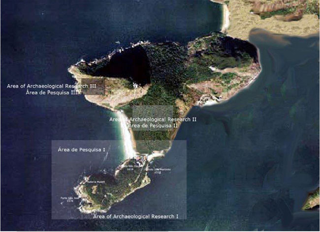
Map of Archaeological Site of Fort St John © Carlos Eduardo Thompson Alves de Souza
Conclusions
The work presented shows methodological suggestions pragmatically without excluding theoretical considerations and focuses on a metropolis. To detect and distinguish objects and human settlement with airborne laser scanner data in urban analysis of ALS data analysis is done by scanning the line instead of the usual approach based on TIN. With the proposed methods, the surfaces can be targeted “on-the-fly”, allowing the ALS can be used in applications that require the processing line data for future work will focus on archeology online detection sites archaeological analysis in urban environments with airborne laser scanning.
Acknowledgements
Ministry of Culture of the Brazilian Government.
References
- Gaspar, M.D. Os próximos passos… Aperfeiçoar a prospecção arqueológica e abrir a caixa do passado. Bol. Mus. Para. Emílio Goeldi. Cienc. Hum, Belém, 6(1): 41-55, 2011
- Anais VIII Simpósio Brasileiro de Sensoriamento Remoto, Salvador, Brasil, 14-19 abril 1996, INPE, p. 899-904. Correções Radiométricas dos Dados Sonográficos da Bacia de Campos. LUCIANO EMÍDIO NEVES DA FONSECA. PETROBRAS-Cenpes Cidade Universitária, Quadra 7 – Ilha do Fundão 21910-900 Rio de Janeiro – RJ.
- Airborne LiDAR Systems for Land and Sea-floor Surveys . Anders Ekelund, (Airborne Hydrography AB, Sweden)
- Fish, J. P., Carr, H. A. Sound Underwater Images. Orleans, MA, Lower Cape Publishing, 1990.
- Meeting the Accuracy Challenge in Airborne LiDAR Bathymetry . Gary C. Guenther, A. Grant Cunningham, Paul E. LaRocque, and David J. Reid. Proceedings of EARSeL-SIG-Workshop LIDAR, Dresden/FRG, June 2000.
- Airborne laser scanning: basic relations and formulas . E.P. Baltsavias (Institute of Geodesy and Photogrammetry, ETH-Hoenggerberg, Zurich)
- Airborne laser scanning: existing systems and firms and other resources . E.P. Baltsavias (Institute of Geodesy and Photogrammetry, ETH-Hoenggerberg, Zurich)
- Airborne laser scanning—an introduction and overview . Aloysius Wehr (Institute for Navigation, University of Stuttgart) and Uwe Lohr (TopoSys, Ralensburg)
- Report: ISPRS Comparison of Filters . George Sithole, George Vosselman (Delft University of Technology, The Netherlands)
- Progress in LiDAR sensor technology . Gottfried Mandlburger, Christian Briese, Norbert Pfeifer (Vienna University of Technology, Wien)
- High Resolution Beam forming of SIMRAD EM3000 Multibeam Sonar Data Are Rønhovde (University of Oslo, Department of Informatics, Cand Scient thesis, 1999)
- IHO Standards for Hydrographic Surveys . (5th Edition, February 2008 Special Publication No. 44, Published by the International Hydrographic Bureau Monaco)
- Airborne LiDAR Systems for Land and Sea-floor Surveys. Anders Ekelund, (Airborne Hydrography AB, Sweden)
- EM 3002 Multibeam echo sounder, (Kongsberg Maritime AS, Norway)


